# P-values
```{r setup, echo=FALSE}
knitr::opts_chunk$set(fig.path="ch19-figures/")
if(FALSE){
knitr::knit("index.qmd")
}
```
In this chapter we will explore several data visualizations related to P-values [@P-values]:
* we begin by explaining the concept of a P-value.
* we simulate some data for two-sample T-testing.
* we show how to create a volcano plot to summarize a set of P-values.
* we explain how to convert an overplotted scatterplot into a linked heat map and zoomed scatterplot.
* we end with another heat map of simulated parameter values, with a linked plot which shows the simulated data.
## What is a P-value? {#what-is-p-value}
A P-value is used to measure significance of a statistical test.
P-values can be used in a wide range of tests, but a typical application is testing for difference between two conditions:
* in a medical experiment, does the treatment do better than the control? For example, with a weight loss drug, we would be interested to know if the treatment group weight is significantly less than the control group weight. Say we have 10 people assigned to the control group, and 15 people assigned to the treatment group. Then we could compute a P-value using an un-paired one-sided T-test to evaluate statistical significance (un-paired because each person in the treatment group does not have a corresponding member in the control group).
* in a machine learning experiment, is the neural network more accurate than the linear model? For example, consider a benchmark image classification data set, and evaluation using 5-fold cross-validation. We would have five measures of test accuracy for each of the two learning algorithms (neural network and linear model). Then we could compute a P-value using a paired one-sided T-test to evaluate statistical significance (paired because the fold 1 test accuracy for the linear model has a corresponding fold 1 test accuracy for the neural network, etc).
After computing the measurements (weight of each person or test accuracy of each machine learning algorithm), we can use them as input to `t.test()`, which will compute a P-value (smaller for a more significant difference).
To understand the P-value, we must first adopt the *null hypothesis*: we assume there is no difference between the conditions.
Then, the P-value of the test is defined as the probability that we observe a difference as large as the given measurements, or larger.
Since under the null hypothesis, there is no difference, it is extremely unlikely to see large differences, so that is why small P-values are more significant.
## Simulated data {#p-value-simulated-data}
We begin by simulating data for use with `t.test()`.
Our simulation has four parameters:
* `true_offset` is the true difference between conditions,
* `sd` is the standard deviation of the simulated data,
* `sample` is a sample number (half of samples in one condition, half in the other),
* `trial` is the number of times that we repeat the experiment (for each offset and standard deviation).
The code below uses `CJ()` to define the values of each parameter:
```{r}
library(data.table)
offset_by <- 0.1
sd_by <- 0.1
set.seed(1)
(sim_dt <- CJ(
  true_offset=round(
    seq(-3, 3, by=offset_by),
    ceiling(-log10(offset_by))),
  sd=seq(0.1, 1, by=sd_by),
  sample=seq(0, 9),
  trial=seq_len(100)
)[, let(
  condition = sample %% 2,
  pair = sample %/% 2
)][, let(
  value = rnorm(.N, true_offset*condition, sd)
)][])
```
The result above shows several hundred thousand rows, one for each simulated random normal `value` (with mean depending on `true_offset` and `condition`).
## T-test and volcano plot {#t-test-and-volcano-plot}
In this section we compute T-test results and visualize them using a volcano plot, which is a plot of negative log P-values versus estimated effect sizes.
The test result visualization is called a volcano plot because the typical distribution of points resembles a volcano erupting from the origin upwards to the left and right.
First, we add columns which we will use for visualization:
* `true_tile` is a text string for selecting a combination of one offset and one standard deviation.
* `Condition` is a string indicating the condition (either `zero` or `offset`).
```{r}
sim_dt[, let(
  true_tile=paste(true_offset, sd),
  Condition = ifelse(condition, "offset", "zero")
)]
```
Next, we do a reshape to obtain a table with a column for each condition (`zero` and `offset`).
```{r}
(sim_wide <- dcast(
  sim_dt,
  true_tile + true_offset + sd + trial + pair ~ Condition))
```
The output above shows a table with half as many rows as the previous table.
The code below computes a T-test for each repetition of the simulation:
```{r}
(sim_p <- sim_wide[, {
  t.result <- t.test(zero, offset, var.equal=TRUE)
  with(t.result, data.table(
    p.value,
    mean_zero=estimate[1],
    mean_offset=estimate[2]
  ))
}, by=.(true_tile, true_offset, sd, trial)])
```
The output above has one row for each T-test, and columns for mean difference (`mean_zero`) and `p.value`.
Since there are ten samples per trial, there are ten times fewer rows than the original simulated data table.
Each trial involves a T-test of 5 control/zero samples, versus 5 treatment/offset samples.
Next, we add columns for the volcano plot:
* `diff_means` is the difference between means of the two conditions, sometimes called the "effect size."
* `neg.log10.p` is the negative log-transformed P-value (larger for more significant).
```{r}
sim_p[, let(
  diff_means = mean_offset - mean_zero,
  neg.log10.p = -log10(p.value)
)]
```
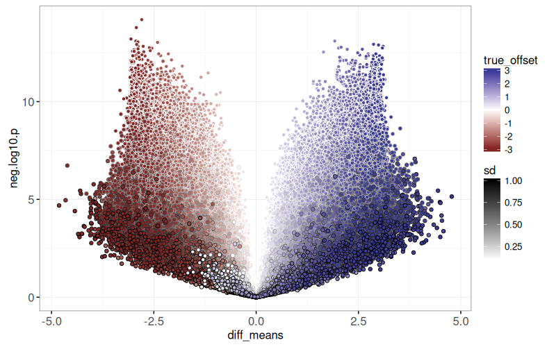
Next, we draw the volcano plot:
* X axis shows the difference between conditions (effect size).
* Y axis shows negative log P-value.
```{r}
library(animint2)
(gg.volcano <- ggplot()+
  geom_point(aes(
    diff_means, neg.log10.p, fill=true_offset, color=sd),
    data=sim_p)+
  scale_fill_gradient2()+
  scale_color_gradient(low="white", high="black")+
  theme_bw())
```
The static graphic above shows one dot per T-test result.
Dots close to the origin (0,0) represent tests which did not yield a significant difference, whereas dots with large Y values represent significant differences.
It also includes `fill=true_offset` and `color=sd` so we can see how the simulation parameters affect the volcano plot:
* Larger `sd` values appear at the bottom (more variance makes it more difficult to detect a difference).
* Darker colors appear near the left/right edges (larger true offsets tend to result in larger computed differences in means).
Finally, the plot above is overplotted, meaning we are unable to see all of the details, because there are too many data points plotted on top of one another.
## Fix overplotting by heat map and zoom {#fix-overplotting-heatmap-zoom}
In this section, we show how the previous volcano plot can be revised to show more detail, using a heat map linked to a zoomed scatterplot.
Note that the computations are an example of pre-aggregation, which is also mentioned in the documentation of altair [@altair] and plotly [@plotly].
To begin, we define the `round_rel()` function below, which is used to add `round_*` and `rel_*` columns which we will use to define heat map tiles.
* `round_*` columns are rounded to the nearest bin size (integer by default), and are used to define the heat map tile `x` and `y` positions.
* `rel_*` columns are used for `x` and `y` positions in the zoomed display, and are units relative to the corresponding `round_*` values.
```{r}
round_rel <- function(DT, col_name, bin_size=1, offset=0){
  value <- DT[[col_name]]
  round_value <- round((value+offset)/bin_size)*bin_size
  DT[, paste0(c("round","rel"), "_", col_name) := list(
    round_value, value-round_value)]
}
round_rel(sim_p, "diff_means")
round_rel(sim_p, "neg.log10.p")
```
Next, we define `volcano_tile`, a text string combination of `round_*` variables, which will be used for selection.
```{r}
sim_p[, volcano_tile := paste(round_diff_means, round_neg.log10.p)]
```
Next, we compute a table with one row per tile in the heat map we will display.
```{r}
(volcano_tile_dt <- sim_p[, .(
  tests=.N
), by=.(volcano_tile, round_diff_means, round_neg.log10.p)])
```
The output above shows one row per heat map tile, with the `tests` column indicating how many points appear in the corresponding area of the volcano plot.
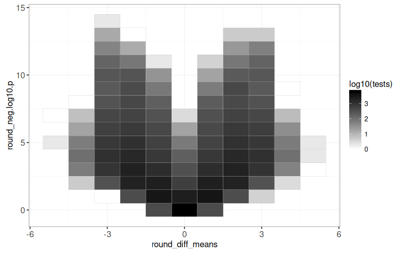
Below we create the volcano heat map.
```{r}
(gg.volcano.tiles <- ggplot()+
  geom_tile(aes(
    round_diff_means, round_neg.log10.p, fill=log10(tests)),
    color="grey",
    data=volcano_tile_dt)+
  scale_fill_gradient(low="white",high="black")+
  theme_bw())
```
The output above is a heat map, with darker regions showing areas of the volcano plot which have more test results.
The code below combines the volcano heat map with a zoomed scatterplot, using the `volcano_tile` selector to link them.
```{r ch19-viz-volcano}
(viz.volcano <- animint(
  volcanoTiles=gg.volcano.tiles+
    ggtitle("Click to select volcano tile")+
    theme_animint(width=300, rowspan=1)+
    geom_tile(aes(
      round_diff_means, round_neg.log10.p),
      clickSelects="volcano_tile",
      color="green",
      fill="transparent",
      data=volcano_tile_dt),
  volcanoZoom=ggplot()+
    ggtitle("Zoom to selected volcano tile")+
    geom_point(aes(
      rel_diff_means, rel_neg.log10.p, fill=true_offset, color=sd),
      showSelected="volcano_tile",
      size=3,
      data=sim_p)+
    scale_fill_gradient2()+
    scale_color_gradient(low="white", high="black")+
    theme_bw()))
```
Above, after clicking the heat map on the left, the data shown in the right plot changes.
## Visualizing grid of simulations {#viz-grid-simulations}
In this section, we create a new visualization to reveal details of each simulation parameter combination.
First, in the code below, we compute the mean effect size (`diff_means`) and negative log P-value (`neg.log10.p`), over all 100 repetitions of each parameter combination.
```{r}
(sim_true_tiles <- dcast(
  sim_p,
  true_tile + true_offset + sd ~ .,
  mean,
  value.var=c("diff_means", "neg.log10.p")))
```
The output above has one row per combination of simulation parameters (`true_offset` and `sd`).
We use the code below to visualize this grid of parameter combinations.
```{r}
width <- offset_by*0.4
height <- sd_by*0.45
(gg.true.tiles <- ggplot()+
  scale_x_continuous("True offset")+
  scale_y_continuous("Standard deviation")+
  scale_fill_gradient2(breaks=c(3,0,-3))+
  scale_color_gradient(
    guide=guide_legend(override.aes=list(fill='white')),
    low="white", high="black", breaks=c(9,5,1))+
  theme_bw()+
  geom_rect(aes(
    xmin=true_offset-width, xmax=true_offset+width,
    ymin=sd-height, ymax=sd+height,
    fill=diff_means, color=neg.log10.p),
    data=sim_true_tiles))
```
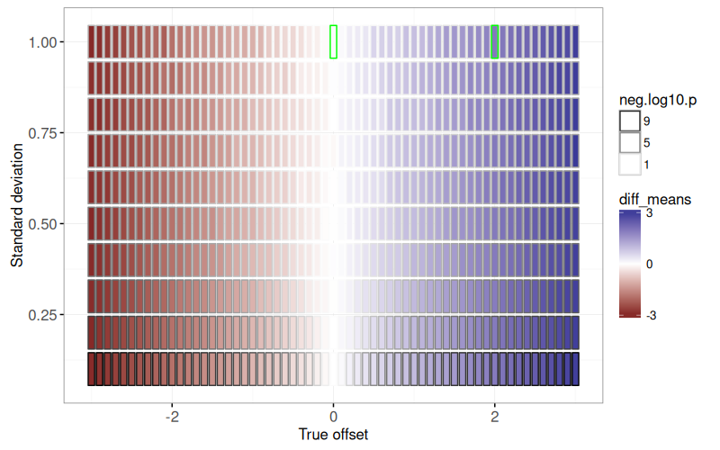
The figure above shows a rectangle for each simulation parameter combination.
It is clear that:
* the estimated effect size (`fill=diff_means`) is consistent with the true offset (X axis).
* the more significant P-values (large `neg.log10.p`) are associated with small standard deviation parameters (because the signal to noise ratio is larger).
We will create a linked plot that shows details of the simulations for each parameter combination.
First we prototype the details plots by examining a subset:
```{r}
some <- function(DT)DT[true_offset %in% c(0,2) & sd == 1]
gg.true.tiles+
  geom_rect(aes(
    xmin=true_offset-width, xmax=true_offset+width,
    ymin=sd-height, ymax=sd+height),
    color="green",
    fill=NA,
    data=some(sim_true_tiles))
```
The figure above shows two rectangles emphasized with a green outline, for which we create a facetted non-interactive plot using the code below.
```{r}
(gg.some.values <- ggplot()+
  facet_grid(true_offset ~ ., labeller=label_both)+
  geom_point(aes(
    trial, value, color=Condition),
    data=some(sim_dt)))
```
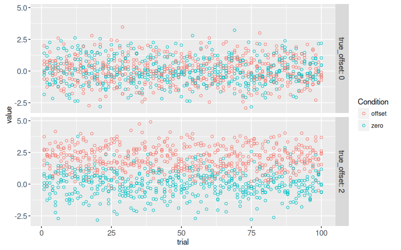
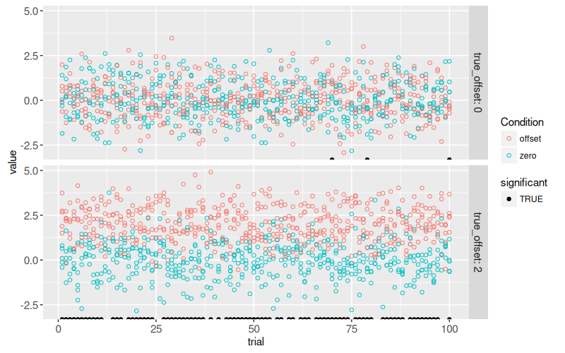
The figure above shows a panel for each of the two parameter combinations emphasized in the previous plot.
The X axis represents `trial`, which ranges from 1 to 100, each one with different random values simulated using the same assumptions (`true_offset=0` or `2`).
The T-test is used to determine if there is any difference in means, between the two conditions.
* When `true_offset=0`, there is no difference between the two conditions, so the T-test should have a small effect size, and a large P-value.
* When `true_offset=2`, there is a larger difference between the two conditions, so the T-test should have a larger effect size, and a small P-value.
The code below creates a new `significant` column which indicates if the test rejects the null hypothesis at the traditional threshold of 5%.
```{r}
sim_p[, significant := p.value < 0.05]
```
The code below adds a new `geom_point()` to emphasize the trials which showed a significant difference at the 5% level.
```{r}
only_significant <- sim_p[significant==TRUE]
gg.some.values+
  geom_point(aes(
    trial, -Inf, fill=significant),
    data=some(only_significant))+
  scale_fill_manual(values=c("TRUE"="black"))
```
The figure above shows a black dot for each trial with a significant difference.
* For `true_offset=0`, we see that there are `r nrow(some(only_significant)[true_offset==0])` trials with a significant difference, even though there is no difference in the true means in the simulation. This number of false positives is consistent with the 5% P-value threshold (type I error rate) that we used to define significance.
* For `true_offset=2`, we see that only `r nrow(some(only_significant)[true_offset!=0])` of the trials are significant, even though there is a true difference in means. The estimated power (true positive rate) is therefore `r some(sim_p)[true_offset!=0, paste0(100*mean(significant),"%")]` and the type II error rate (false negative rate) is therefore `r some(sim_p)[true_offset!=0, paste0(100*mean(1-significant),"%")]`.
Below we create a visualization which links the overview heat map to the details scatter plot, by replacing `facet_grid(true_offset ~ .)` in the code above, with `showSelected="true_tile"` in the code below.
```{r ch19-viz-true-tiles}
(viz.parameters <- animint(
  tiles=gg.true.tiles+
    ggtitle("Click to select simulation parameters")+
    theme_animint(width=800, height=250, last_in_row=TRUE)+
    geom_rect(aes(
      xmin=true_offset-width, xmax=true_offset+width,
      ymin=sd-height, ymax=sd+height),
      fill="transparent",
      color="green",
      clickSelects="true_tile",
      data=sim_true_tiles),
  zoom=ggplot()+
    ggtitle("Zoom to selected simulation parameters")+
    theme_bw()+
    theme_animint(width=800, height=300)+
    geom_point(aes(
      trial, value, color=Condition),
      fill=NA,
      showSelected="true_tile",
      data=sim_dt)+
    geom_point(aes(
      trial, -Inf, fill=significant),
      showSelected="true_tile",
      data=only_significant)+
    scale_fill_manual(values=c("TRUE"="black"))))
```
In the visualization above, you can click on the top plot to select a simulation parameter combination.
The 100 trials for the selected parameter combination are shown in the bottom plot.
## Chapter summary and exercises {#ch19-exercises}
We have created several data visualizations using simulations to illustrate P-values.
Since there were too many T-tests to show on the volcano plot, we instead used a heat map linked to a zoomed scatter plot.
We also showed how to link a heat map of parameter combinations to a scatter plot which shows details of the corresponding values in the simulations.
Exercises:
* In `viz.volcano`, when clicking on one of the bottom `volcanoTiles`, we see only have of the space occupied in `volcanoZoom`. To fix this, and have all of the space occupied, go back to the definition of `round_neg.log10.p`, and use the `offset=0.5` argument in `round_rel()`, which will shift the relative values by a certain offset.
* In `viz.volcano`, add `aes(tooltip)` to `volcanoTiles` to show how many points are in each heat map tile.
* Note how two `geom_tile()` were used in `viz.volcano`, and two `geom_rect()` were used in `viz.parameters`. The first geom uses color and fill to visualize the data, whereas the second geom uses `fill="transparent"` with `color="green"` for selection. Try a re-design with only one geom, which only uses `aes(fill)` and instead uses `color` as a geom parameter. What are the disadvantages of the approach using only one geom?
* In `viz.parameters`, add `geom_hline()` to emphasize the selected value of the true offset.
* In `viz.parameters$zoom`, add `geom_segment()` to represent the difference between means in each trial, using `aes(linetype=signficant)` to show which differences are significant at the traditional P-value threshold of `0.05`.
* In `viz.parameters$zoom`, add `geom_point()` to represent the mean in each trial and condition. Hint: you can either add two instances of `geom_point()`, or one `geom_point()` with a longer data table created via `melt(sim_p, measure.vars=measure(Condition, sep="mean_(.*)"))`.
* Add graphical elements to `gg.volcano` to emphasize the traditional P-value threshold of `0.05`: `geom_hline()` can show the threshold, and `geom_text()` can show how many tests fall above or below the threshold (use text like "1500 tests not significant").
* Add `aes(tooltip)` to `gg.true.tiles` to show values of `neg.log10.p` and `diff_means`.
* Add animation to `viz.parameters` so that we see a new parameter combination every second.
* Add `first` option to `viz.parameters` so that the first selection we see is the same as one of the parameter combinations shown in the static facetted plot.
* Combine `viz.volcano` with `viz.parameters` to create a new data visualization with four linked plots. Different kinds of interactions are possible:
* In `volcanoZoom`, use `clickSelects="true_tile"` so that interactivity can be used to map volcano plot points back into the simulation parameter space. Add green dots with `showSelected="true_tile"` to `volcanoTiles` to show where the 100 trials for the selected parameter combination appear in volcano plot space.
* Create a new selection variable that is a unique combination of `true_tile` and `trial`, then use it for `clickSelects` in both `volcanoZoom` and `viz.parameters$zoom`, so that we can see a correspondence between a point in volcano space, and a trial in the parameter zoom details plot.
Next, [Chapter 20](/ch20) explains how to visualize results of machine learning benchmarks.