tryCatch({
  data(montreal.bikes, package="animint2")
}, warning=function(w){
  remotes::install_github("tdhock/animint2")
})9 Montreal bikes
In this chapter we will explore several data visualizations of the Montreal bike data set.
Chapter outline:
- We begin with some static data visualizations.
- We create an interactive visualization of accident frequency over time.
- We create a interactive data viz with four plots, showing monthly accident trends, daily details, and a map of counter locations.
9.1 Static figures
We begin by loading the montreal.bikes data set, which is not available in the CRAN release of animint2, in order to save space on CRAN. Therefore to access this data set, you will need to install animint2 from GitHub:
We begin by examining the accidents data table.
library(animint2)
data(montreal.bikes) #only present if installed from github
old.locale <- Sys.setlocale(locale="en_US.UTF-8")
for(col_name in c("nom","nom_comptage","Etat")){
  montreal.bikes$counter.locations[[col_name]] <- iconv(
    montreal.bikes$counter.locations[[col_name]], "latin1", "UTF-8")
}
library(data.table)
accidents.dt <- data.table(montreal.bikes$accidents)
accidents.dt[1]
date.str time.str deaths people.severely.injured people.slightly.injured
1: 2012-01-02 18:35 0 0 1
street.number street cross.street location.int position.int
1: NA ST JEAN BAPTISTE O AV ROULEAU 32 6
position location
1: Voie de circulation En intersection (moins de 5 mètres)Each accident has data about its date, time, location, and counts of death and slight/severe injury. Some of the values are in French (e.g. position Voie de circulation, location En intersection, etc).
We calculate the time period of the accidents below.
(accidents.dt[
, date.POSIXct := as.POSIXct(strptime(date.str, "%Y-%m-%d"))
][
, month.str := strftime(date.POSIXct, "%Y-%m")
][])
date.str time.str deaths people.severely.injured
1: 2012-01-02 18:35 0 0
2: 2012-01-05 21:50 0 0
---
5594: 2014-12-27 12:35 0 0
5595: 2014-12-30 11:55 0 0
people.slightly.injured street.number street cross.street
1: 1 NA ST JEAN BAPTISTE O AV ROULEAU
2: 1 NA FOSTER JANELLE
---
5594: 1 NA CH DES PATRIOTES 1RE RUE
5595: 1 14965 PIERREFONDS BD JACQUES BIZARD
location.int position.int position
1: 32 6 Voie de circulation
2: 34 6 Voie de circulation
---
5594: 33 6 Voie de circulation
5595: 33 5 Voie cyclable / chaussée désignée
location date.POSIXct month.str
1: En intersection (moins de 5 mètres) 2012-01-02 2012-01
2: Entre intersections (100 mètres et +) 2012-01-05 2012-01
---
5594: Près d'une intersection/carrefour giratoire 2014-12-27 2014-12
5595: Près d'une intersection/carrefour giratoire 2014-12-30 2014-12range(accidents.dt$month.str)[1] "2012-01" "2014-12"Below we also compute the range of months for the bike counter data table.
(counts.dt <- data.table(montreal.bikes$counter.counts)) location date count
1: Berri 2009-01-01 05:00:00 29
2: Berri 2009-01-02 05:00:00 19
---
13382: Totem_Laurier 2013-09-17 04:00:00 3745
13383: Totem_Laurier 2013-09-18 04:00:00 3921[1] "2009-01" "2013-09"The bike counts are time series data which we visualize below.
counts.dt[, loc.lines := gsub("[- _]", "\n", location)]
ggplot()+
  theme_bw()+
  theme(panel.margin=grid::unit(0, "lines"))+
  facet_grid(loc.lines ~ .)+
  geom_point(aes(
    date, count, color=count==0),
    shape=21,
    data=counts.dt)+
  scale_color_manual(values=c("TRUE"="grey", "FALSE"="black"))
Warning: Removed 407 rows containing missing values (geom_point).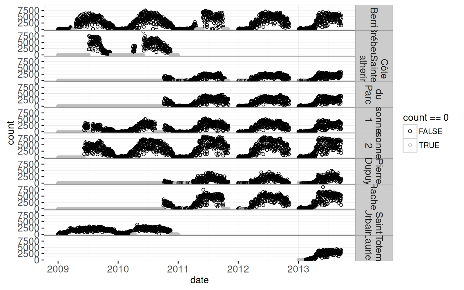
Plotting with geom_point makes it easy to see the difference between zeros and missing values.
We will compute a summary of all accidents per month in this time period, so we first create a data table for each month below. (and make sure to set the locale to C for English month names)
uniq.month.vec <- unique(c(
  accidents.dt$month.str,
  counts.dt$month.str))
one.day <- 60 * 60 * 24
months <- data.table(month.str=uniq.month.vec)[
, month01.str := paste0(month.str, "-01")
][
, month01.POSIXct := as.POSIXct(strptime(month01.str, "%Y-%m-%d"))
][, let(
  next.POSIXct = month01.POSIXct + one.day * 31,
  month.str = strftime(month01.POSIXct, "%B %Y")
)][
, next01.str := paste0(strftime(next.POSIXct, "%Y-%m"), "-01")
][
, next01.POSIXct := as.POSIXct(strptime(next01.str, "%Y-%m-%d"))
]
month.levs <- months[order(month01.POSIXct), month.str]
(months[, month := factor(month.str, month.levs)][])
month.str month01.str month01.POSIXct next.POSIXct next01.str
1: January 2012 2012-01-01 2012-01-01 2012-02-01 2012-02-01
2: February 2012 2012-02-01 2012-02-01 2012-03-03 2012-03-01
---
71: November 2011 2011-11-01 2011-11-01 2011-12-02 2011-12-01
72: December 2011 2011-12-01 2011-12-01 2012-01-01 2012-01-01
next01.POSIXct month
1: 2012-02-01 January 2012
2: 2012-03-01 February 2012
---
71: 2011-12-01 November 2011
72: 2012-01-01 December 2011Note that we created a month column which is a factor ordered by month.levs.
month_pos_ct <- function(mstr)as.POSIXct(
  strptime(paste0(mstr, "-15"), "%Y-%m-%d"))
accidents.dt[
, month.text := strftime(date.POSIXct, "%B %Y")
][
, month := factor(month.text, month.levs)
][
, month.POSIXct := month_pos_ct(month.str)
][]
date.str time.str deaths people.severely.injured
1: 2012-01-02 18:35 0 0
2: 2012-01-05 21:50 0 0
---
5594: 2014-12-27 12:35 0 0
5595: 2014-12-30 11:55 0 0
people.slightly.injured street.number street cross.street
1: 1 NA ST JEAN BAPTISTE O AV ROULEAU
2: 1 NA FOSTER JANELLE
---
5594: 1 NA CH DES PATRIOTES 1RE RUE
5595: 1 14965 PIERREFONDS BD JACQUES BIZARD
location.int position.int position
1: 32 6 Voie de circulation
2: 34 6 Voie de circulation
---
5594: 33 6 Voie de circulation
5595: 33 5 Voie cyclable / chaussée désignée
location date.POSIXct month.str
1: En intersection (moins de 5 mètres) 2012-01-02 2012-01
2: Entre intersections (100 mètres et +) 2012-01-05 2012-01
---
5594: Près d'une intersection/carrefour giratoire 2014-12-27 2014-12
5595: Près d'une intersection/carrefour giratoire 2014-12-30 2014-12
month.text month month.POSIXct
1: January 2012 January 2012 2012-01-15
2: January 2012 January 2012 2012-01-15
---
5594: December 2014 December 2014 2014-12-15
5595: December 2014 December 2014 2014-12-15stopifnot(!is.na(accidents.dt$month.POSIXct))
accidents.per.month <- accidents.dt[, list(
total.accidents=.N,
total.people=sum(
deaths+people.severely.injured+people.slightly.injured),
deaths=sum(deaths),
people.severely.injured=sum(people.severely.injured),
people.slightly.injured=sum(people.slightly.injured),
next.POSIXct = month.POSIXct + one.day * 30,
month01.str = paste0(strftime(month.POSIXct, "%Y-%m"), "-01")
), by=.(month, month.str, month.text, month.POSIXct)][, let(
month01.POSIXct = as.POSIXct(strptime(month01.str, "%Y-%m-%d")),
next01.str = paste0(strftime(next.POSIXct, "%Y-%m"), "-01")
)][
, next01.POSIXct := as.POSIXct(strptime(next01.str, "%Y-%m-%d"))
][]We plot the accidents per month below.
accidents.tall <- melt(
  accidents.per.month,
  measure.vars=c(
    "deaths", "people.severely.injured", "people.slightly.injured"),
  variable.name="severity",
  value.name="people")
severity.colors <- c(
  deaths="#A50F15",#dark red
  people.severely.injured="#FB6A4A",
  people.slightly.injured="#FEE0D2")#lite red
ggplot()+
  theme_bw()+
  geom_bar(aes(
    month.POSIXct, people, fill=severity),
    stat="identity",
    data=accidents.tall)+
  scale_fill_manual(values=severity.colors)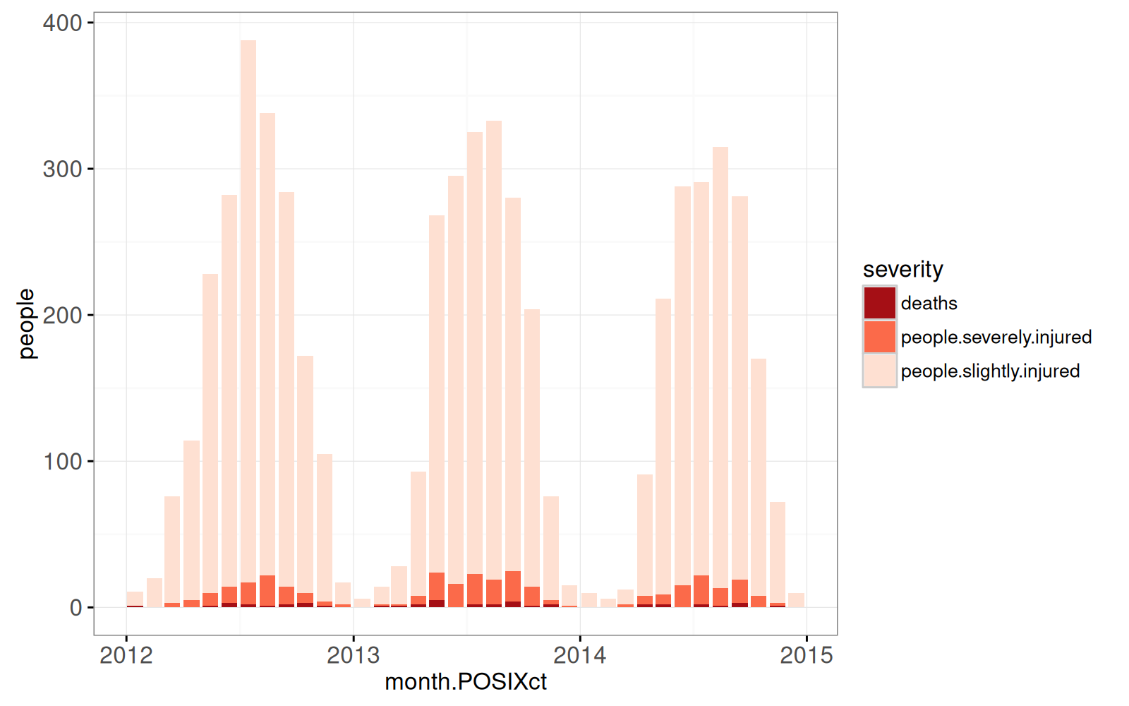
In each accident, there are counts of people who died, along with people who suffered severe and slight injuries. Below we classify the severity of each accident according to the worst outcome among the people affected.
severity
                 deaths people.severely.injured people.slightly.injured
                     44                     289                    5262
The output above shows that accidents with only slight injuries are most frequent, and accidents with at least one death are least frequent. Below we compute counts per month.
counts.per.month <- counts.dt[, let(
  month.POSIXct = month_pos_ct(month.str),
  month.text = strftime(date, "%B %Y"),
  day.of.the.month = as.integer(strftime(date, "%d"))
)][
, month := factor(month.text, month.levs)
][, list(
  days=.N,
  mean.per.day=mean(count),
  count=sum(count),
  month01.str = paste0(month.str, "-01")
), by=.(location, month, month.str, month.POSIXct)][
  0 < count
][
, month01.POSIXct := as.POSIXct(strptime(month01.str, "%Y-%m-%d"))
][
, next.POSIXct := month01.POSIXct + one.day * 31
][
, next01.str := paste0(strftime(next.POSIXct, "%Y-%m"), "-01")
][
, next01.POSIXct := as.POSIXct(strptime(next01.str, "%Y-%m-%d"))
][
, days.in.month := as.integer(round(difftime(next01.POSIXct,month01.POSIXct,units="days")))
][]
counts.per.month[days < days.in.month, {
  list(location, month, days, days.in.month)
}]
location month days days.in.month
1: Berri November 2012 5 30
2: Côte-Sainte-Catherine November 2012 5 30
---
14: Rachel September 2013 18 30
15: Totem_Laurier September 2013 18 30As shown above, some months do not have observations for all days.
9.2 Interactive viz of accident frequency
complete.months <- counts.per.month[days == days.in.month]
month.labels <- counts.per.month[, {
  .SD[which.max(count), ]
}, by=location]
day.labels <- counts.dt[, {
  .SD[which.max(count), ]
}, by=.(location, month)]
city.wide.cyclists <- counts.per.month[0 < count, list(
  locations=.N,
  count=sum(count),
  month01.str = paste0(month.str, "-01")
), by=.(month, month.str, month.POSIXct)][
, month01.POSIXct := as.POSIXct(strptime(month01.str, "%Y-%m-%d"))
][
, next.POSIXct := month01.POSIXct + one.day * 31
][
, next01.str := paste0(strftime(next.POSIXct, "%Y-%m"), "-01")
][
, next01.POSIXct := as.POSIXct(strptime(next01.str, "%Y-%m-%d"))
][]
month.str.vec <- strftime(seq(
  strptime("2012-01-15", "%Y-%m-%d"),
  strptime("2013-01-15", "%Y-%m-%d"),
  by="month"), "%Y-%m")
city.wide.complete <- complete.months[0 < count, list(
  locations=.N,
  count=sum(count),
  month01.str = paste0(month.str, "-01")
), by=.(month, month.str, month.POSIXct)]
setkey(city.wide.complete, month.str)
scatter.cyclists <- city.wide.complete[month.str.vec]
scatter.accidents <- accidents.per.month[
  scatter.cyclists, on=.(month.str)]
scatter.not.na <- scatter.accidents[!is.na(locations),]
scatter.max <- scatter.not.na[locations==max(locations)]
fit <- lm(total.accidents ~ count - 1, scatter.max)
scatter.max[, pred.accidents := predict(fit)]
animint(
  regression=ggplot()+
    theme_bw()+
    ggtitle("Numbers of accidents and cyclists")+
    geom_line(aes(
      count, pred.accidents),
      color="grey",
      data=scatter.max)+
    geom_point(aes(
      count, total.accidents),
      shape=1,
      clickSelects="month",
      size=5,
      alpha=0.75,
      data=scatter.max)+
    ylab("Total bike accidents (all Montreal locations)")+
    xlab("Total cyclists (all Montreal locations)"),
  timeSeries=ggplot()+
    theme_bw()+
    ggtitle("Time series of accident frequency")+
    xlab("Month")+
    geom_point(aes(
      month.POSIXct, total.accidents/count),
      clickSelects="month",
      size=5,
      alpha=0.75,
      data=scatter.max))
The data viz above shows two data visualizations of city-wide accident frequency over time. The plot on the left shows that the number of accidents grows with the number of cyclists. The plot on the right shows the frequency of accidents over time.
9.3 Interactive viz with map and details
The plot below is a dotplot of accidents for each month. Each dot represents one person who got in an accident.
accidents.cumsum <- accidents.dt[
  order(date.POSIXct, month, severity)
][
, accident.i := seq_along(severity)
, by=.(date.POSIXct, month)
][
, day.of.the.month := as.integer(strftime(date.POSIXct, "%d"))
][]
ggplot()+
  theme_bw()+
  theme(panel.margin=grid::unit(0, "cm"))+
  facet_wrap("month")+
  geom_text(aes(15, 25, label=month), data=accidents.per.month)+
  scale_fill_manual(values=severity.colors, breaks=rev(names(severity.colors)))+
  scale_x_continuous("day of the month", breaks=c(1, 10, 20, 30))+
  geom_point(aes(
    day.of.the.month, accident.i, fill=severity),
    shape=21,
    data=accidents.cumsum)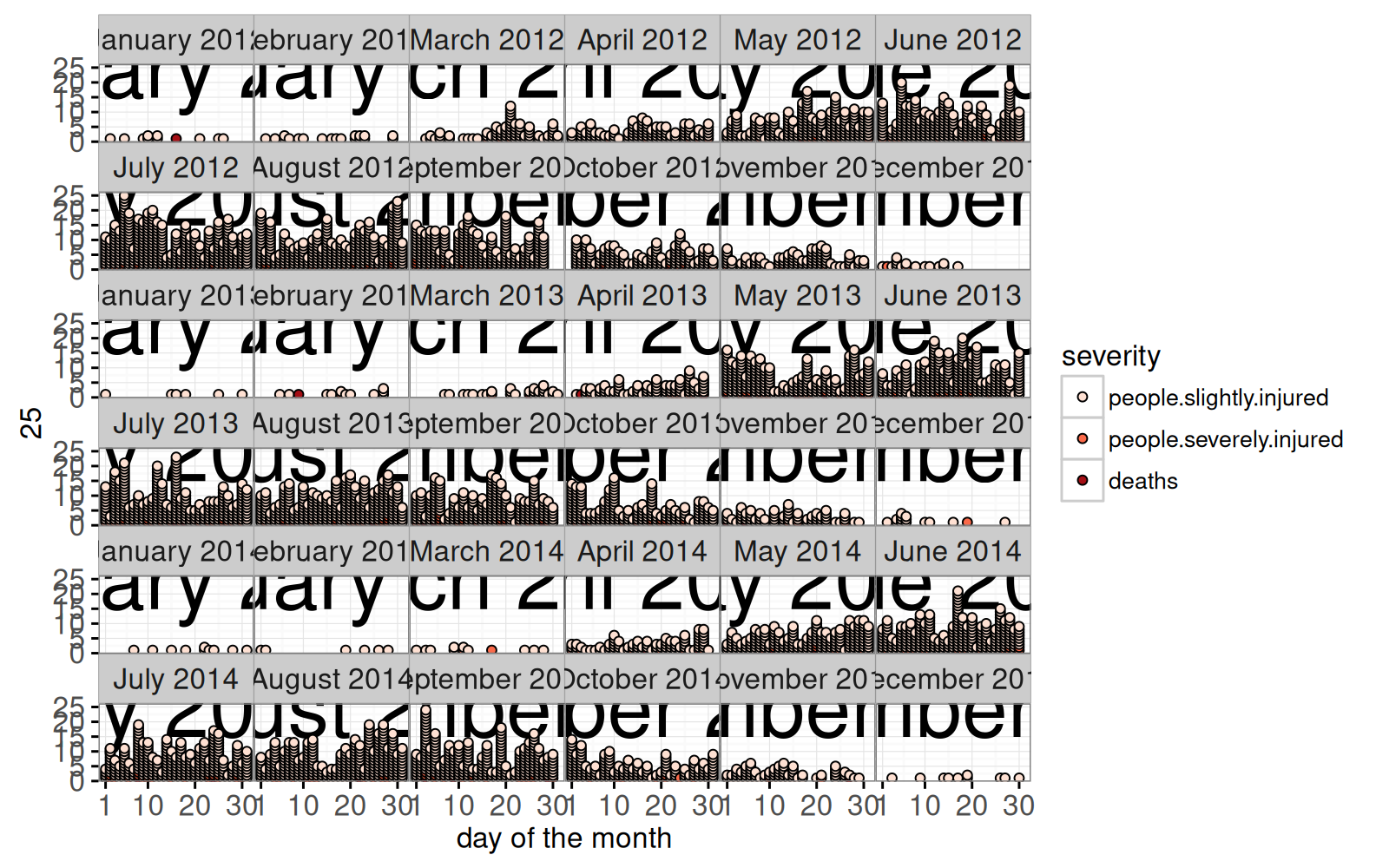
counter.locations <- data.table(
  montreal.bikes$counter.locations
)[, let(
  lon = coord_X,
  lat = coord_Y
)][]
loc.name.code <- c(
  "Berri1"="Berri",
  "Brebeuf"="Brébeuf",
  CSC="Côte-Sainte-Catherine",
  "Maisonneuve_1"="Maisonneuve 1",
  "Maisonneuve_2"="Maisonneuve 2",
  "Parc"="du Parc",
  PierDup="Pierre-Dupuy",
  "Rachel/Papineau"="Rachel",
  "Saint-Urbain"="Saint-Urbain",
  "Totem_Laurier"="Totem_Laurier")
counter.locations[, location := loc.name.code[nom_comptage] ]
velo.counts <- table(counts.dt$location)
(show.locations <- counter.locations[
  names(velo.counts), on=.(location)])
id nom nom_comptage Etat Type
1: 3 Berri_1 Berri1 Existant compteur
2: 2 Brebeuf_1 Brebeuf Existant compteur
3: 8 Cote-Ste-Catherine_1 CSC Existant compteur
4: 4 Maisonneuve_1 Maisonneuve_1 À réinstaller compteur
5: 5 Maisonneuve_2 Maisonneuve_2 Existant compteur
6: 22 Parc_1 Parc Existant compteur
7: 12 Pierre-Dupuy_1 PierDup Existant compteur
8: 6 Rachel/Papineau Rachel/Papineau Existant compteur
9: 1 St-Urbain_1 Saint-Urbain Existant compteur
10: 37 Totem_Laurier Totem_Laurier Existant totem
Annee_implante coord_X coord_Y lon lat location
1: 2008 -73.56284 45.51613 -73.56284 45.51613 Berri
2: 2009 -73.57398 45.52741 -73.57398 45.52741 Brébeuf
3: 2010 -73.60783 45.51496 -73.60783 45.51496 Côte-Sainte-Catherine
4: 2008 -73.56159 45.51479 -73.56159 45.51479 Maisonneuve 1
5: 2008 -73.57508 45.50054 -73.57508 45.50054 Maisonneuve 2
6: 2010 -73.58171 45.51346 -73.58171 45.51346 du Parc
7: 2010 -73.54455 45.49966 -73.54455 45.49966 Pierre-Dupuy
8: 2007 -73.56965 45.53036 -73.56965 45.53036 Rachel
9: 2014 -73.58888 45.51955 -73.58888 45.51955 Saint-Urbain
10: 2013 -73.58883 45.52777 -73.58883 45.52777 Totem_LaurierThe counter locations above will be plotted below. Note that we use showSelected=month and clickSelects=location.
map.lim <- show.locations[, list(
  range.lat=range(lat),
  range.lon=range(lon)
)]
diff.vec <- sapply(map.lim, diff)
diff.mat <- c(-1, 1) * matrix(diff.vec, 2, 2, byrow=TRUE)
scale.mat <- as.matrix(map.lim) + diff.mat
location.colors <-
  c("#8DD3C7", "#FFFFB3", "#BEBADA", "#FB8072", "#80B1D3", "#FDB462",
    "#B3DE69", "#FCCDE5", "#D9D9D9", "#BC80BD", "#CCEBC5", "#FFED6F")
names(location.colors) <- show.locations$location
counts.per.month.loc <- counts.per.month[
  show.locations, on=.(location)]
bike.paths <- data.table(montreal.bikes$path.locations)
some.paths <- bike.paths[
  scale.mat[1, "range.lat"] < lat &
    scale.mat[1, "range.lon"] < lon &
    lat < scale.mat[2, "range.lat"] &
    lon < scale.mat[2, "range.lon"]]
mtl.map <- ggplot()+
  theme_bw()+
  theme(
    panel.margin=grid::unit(0, "lines"),
    axis.line=element_blank(), axis.text=element_blank(),
    axis.ticks=element_blank(), axis.title=element_blank(),
    panel.background = element_blank(),
    panel.border = element_blank())+
  coord_equal(xlim=map.lim$range.lon, ylim=map.lim$range.lat)+
  scale_color_manual(values=location.colors)+
  scale_x_continuous(limits=scale.mat[, "range.lon"])+
  scale_y_continuous(limits=scale.mat[, "range.lat"])+
  geom_path(aes(
    lon, lat,
    tooltip=TYPE_VOIE,
    group=paste(feature.i, path.i)),
    color="grey",
    data=some.paths)+
  guides(color="none")+
  geom_text(aes(
    lon, lat,
    label=location),
    clickSelects="location",
    data=show.locations)
mtl.map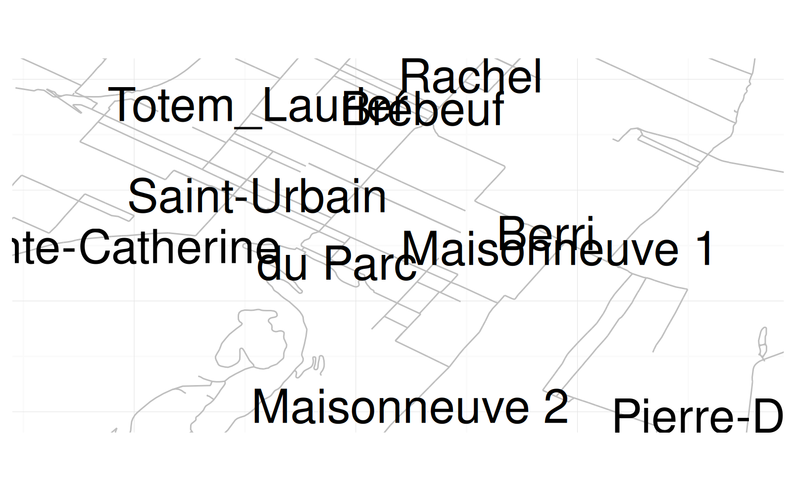
The plot below shows the time period that each counter was in operation. Note that we use geom_tallrect with clickSelects to select the month.
location.ranges <- counts.per.month[0 < count, list(
  min=min(month.POSIXct),
  max=max(month.POSIXct)
), by=location]
accidents.range <- accidents.dt[, data.table(
  location="accidents",
  min=min(date.POSIXct),
  max=max(date.POSIXct))]
MonthSummary <- ggplot()+
  theme_bw()+
  theme_animint(width=450, height=250)+
  xlab("range of dates in data")+
  ylab("data type")+
  scale_color_manual(values=location.colors)+
  guides(color="none")+
  geom_segment(aes(
    min, location,
    xend=max, yend=location,
    color=location),
    clickSelects="location",
    data=location.ranges, alpha=3/4, size=10)+
  geom_segment(aes(
    min, location,
    xend=max, yend=location),
    color=severity.colors[["deaths"]],
    data=accidents.range,
    size=10)
MonthSummary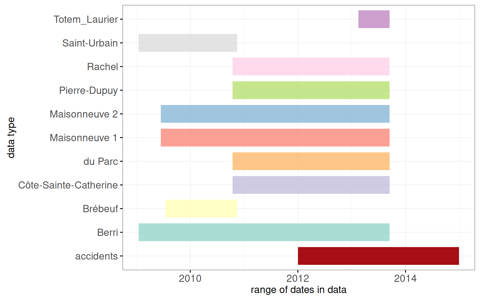
The plot below shows the bike counts at each location and day.
                     date            min.date            max.date locations
   1: 2009-01-01 05:00:00 2008-12-31 17:00:00 2009-01-01 17:00:00         9
   2: 2009-01-02 05:00:00 2009-01-01 17:00:00 2009-01-02 17:00:00         9
  ---
1607: 2013-09-17 04:00:00 2013-09-16 16:00:00 2013-09-17 16:00:00         8
1608: 2013-09-18 04:00:00 2013-09-17 16:00:00 2013-09-18 16:00:00         8
location.labels <- counts.dt[
, .SD[which.max(count)]
, by=list(location)]
TimeSeries <- ggplot()+
theme_bw()+
geom_tallrect(aes(
xmin=date-one.day/2, xmax=date+one.day/2,
clickSelects=date),
data=dates, alpha=1/2)+
geom_line(aes(
date, count, group=location,
showSelected=location,
clickSelects=location),
data=counts.dt)+
scale_color_manual(values=location.colors)+
geom_point(aes(
date, count, color=location,
showSelected=location,
clickSelects=location),
data=counts.dt)+
geom_text(aes(
date, count+200, color=location, label=location,
showSelected=location,
clickSelects=location),
data=location.labels)
TimeSeriesWarning: Removed 407 rows containing missing values (geom_point).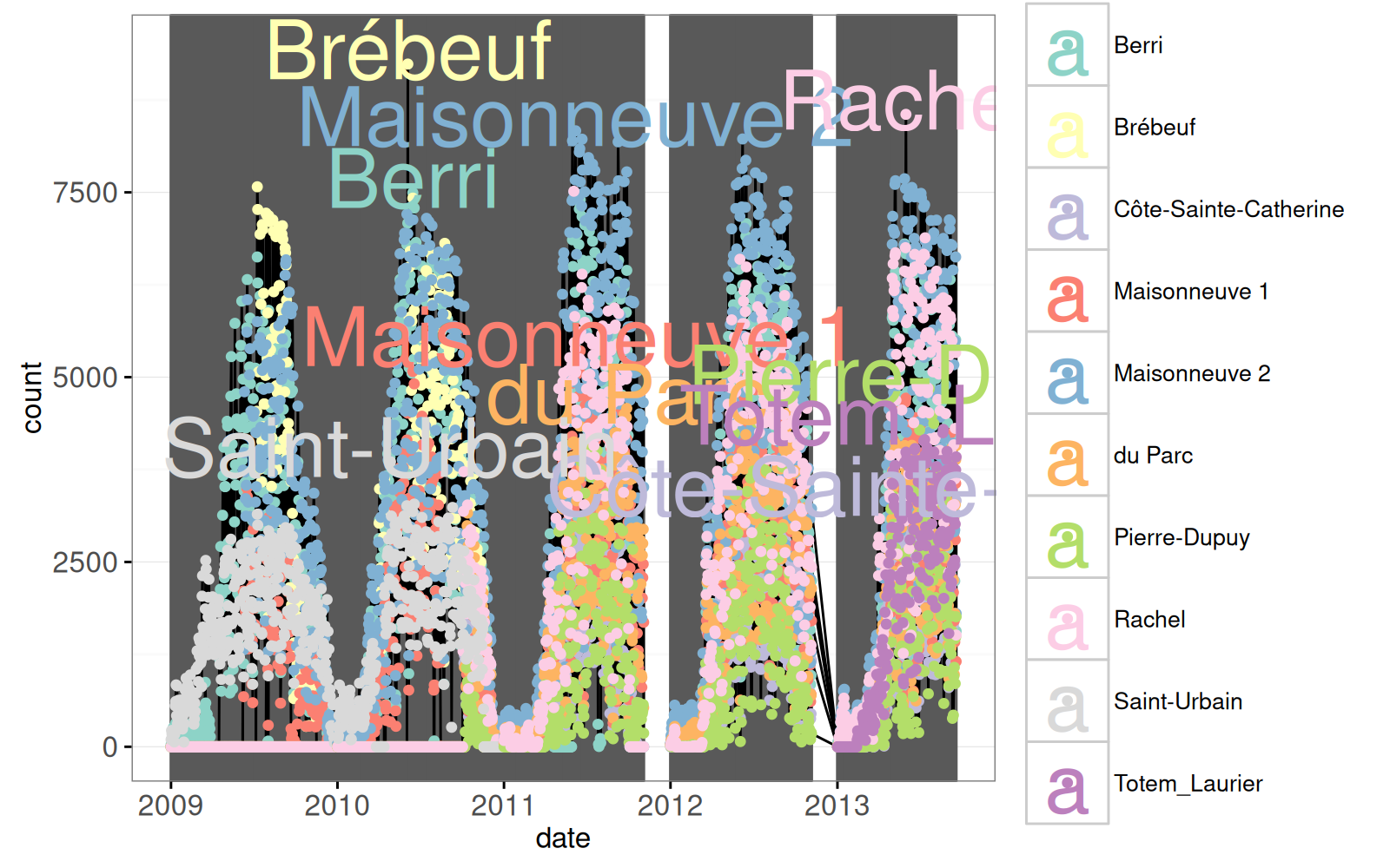
The plot below shows the same data but for each month.
MonthSeries <- ggplot()+
  guides(color="none", fill="none")+
  theme_bw()+
  geom_tallrect(aes(
    xmin=month01.POSIXct, xmax=next01.POSIXct),
    clickSelects="month",
    data=months,
    alpha=1/2)+
  geom_line(aes(
    month.POSIXct, count, group=location,
    color=location),
    showSelected="location",
    clickSelects="location",
    data=counts.per.month)+
  scale_color_manual(values=location.colors)+
  scale_fill_manual(values=location.colors)+
  xlab("month")+
  ylab("bike counts per month")+
  geom_point(aes(
    month.POSIXct, count, fill=location,
    tooltip=paste(
      count, "bikers counted at",
      location, "in", month)),
    showSelected="location",
    clickSelects="location",
    size=5,
    color="black",
    data=counts.per.month)+
  geom_text(aes(
    month.POSIXct, count+5000, color=location, label=location),
    showSelected="location",
    clickSelects="location",
    data=month.labels)
MonthSeries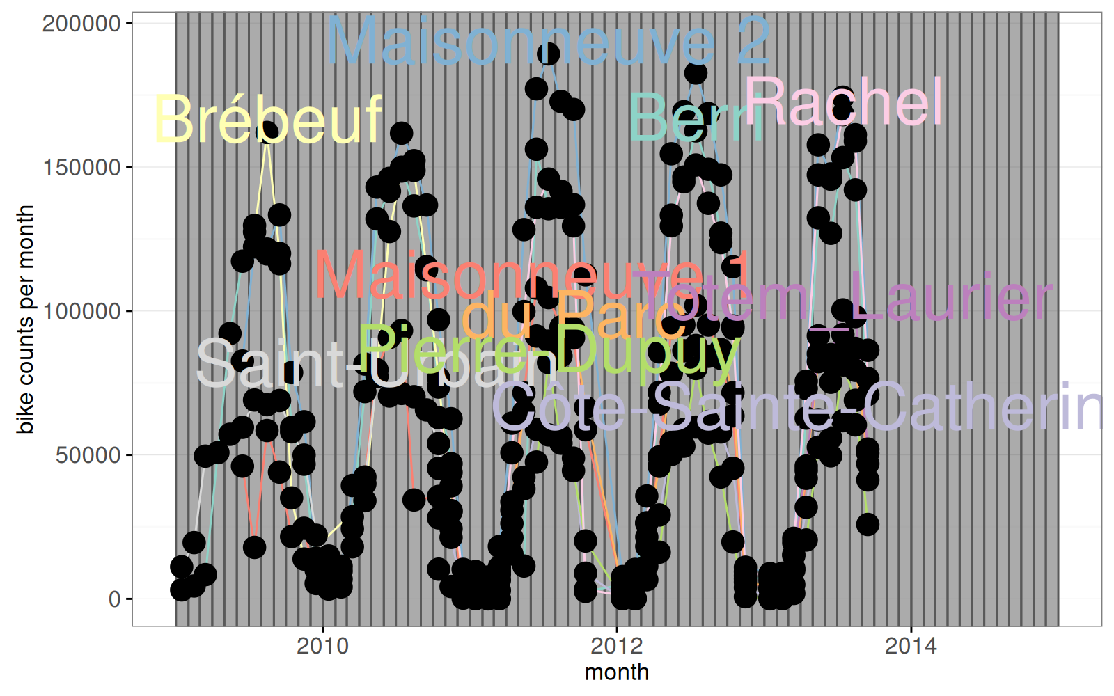
counter.title <- "mean cyclists/day"
accidents.title <- "city-wide accidents"
person_people <- function(num, suffix)ifelse(
  num==0, "",
  sprintf(
    "%d %s %s",
    num,
    ifelse(num==1, "person", "people"),
    suffix))
deaths_severe_slight <- function(deaths, severe, slight)apply(cbind(
  ifelse(
    deaths==0, "",
    sprintf(
      "%d death%s",
      deaths,
      ifelse(deaths==1, "", "s"))),
  person_people(severe, "severely injured"),
  person_people(slight, "slightly injured")),
  1, function(x)paste(x[x!=""], collapse=", "))
MonthFacet <- ggplot()+
  ggtitle("All data, select month")+
  guides(color="none", fill="none")+
  theme_bw()+
  facet_grid(facet ~ ., scales="free")+
  theme(panel.margin=grid::unit(0, "lines"))+
  geom_tallrect(aes(
    xmin=month01.POSIXct, xmax=next01.POSIXct),
    clickSelects="month",
    data=data.table(
      city.wide.cyclists,
      facet=counter.title),
    alpha=1/2)+
  geom_line(aes(
    month.POSIXct, mean.per.day, group=location,
    color=location),
    showSelected="location",
    clickSelects="location",
    data=data.table(counts.per.month, facet=counter.title))+
  scale_color_manual(values=location.colors)+
  xlab("month")+
  ylab("")+
  geom_point(aes(
    month.POSIXct, mean.per.day, color=location,
    tooltip=paste(
      count, "cyclists counted at",
      location, "in",
      days, "days of", month,
      sprintf("(mean %d cyclists/day)", as.integer(mean.per.day)))),
    showSelected="location",
    clickSelects="location",
    size=5,
    fill="grey",
    data=data.table(counts.per.month, facet=counter.title))+
  geom_text(aes(
    month.POSIXct, mean.per.day+300, color=location, label=location),
    showSelected="location",
    clickSelects="location",
    data=data.table(month.labels, facet=counter.title))+
  scale_fill_manual(values=severity.colors)+
  geom_bar(aes(
    month.POSIXct, people,
    fill=severity),
    showSelected="severity",
    stat="identity",
    position="identity",
    color=NA,
    data=data.table(accidents.tall, facet=accidents.title))+
  geom_tallrect(aes(
    xmin=month01.POSIXct, xmax=next01.POSIXct,
    tooltip=paste(
      deaths_severe_slight(
        deaths,
        people.severely.injured,
        people.slightly.injured),
      "in", month)),
    clickSelects="month",
    alpha=0.5,
    data=data.table(accidents.per.month, facet=accidents.title))
MonthFacet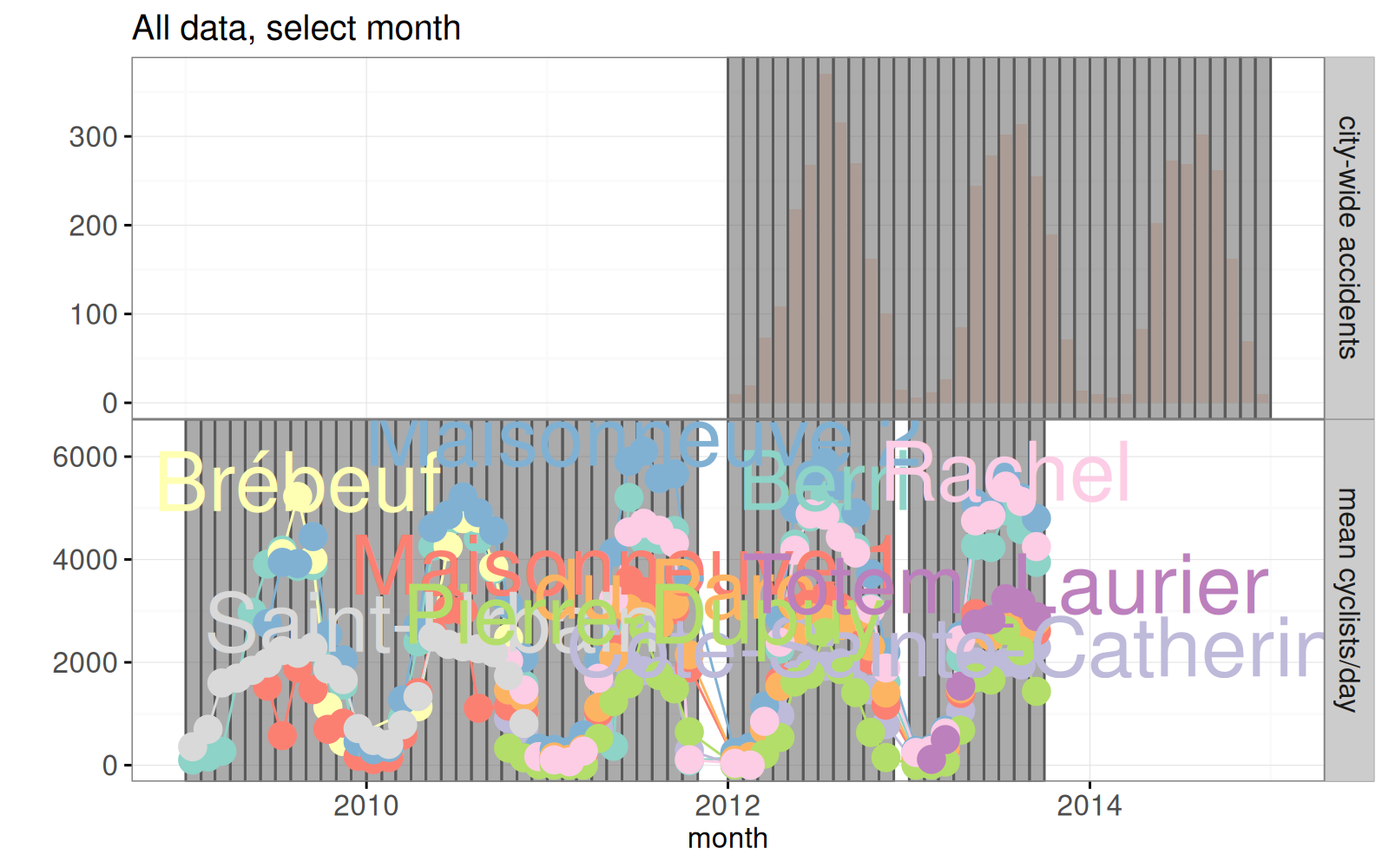
      day.POSIXct day.of.the.week
   1:  2009-01-01             Thu
   2:  2009-01-02             Fri
  ---
2191:  2014-12-31             Wed
2192: 2015-01-01 Thu day.POSIXct day.of.the.week month.text day.of.the.month month
1: 2009-01-03 Sat January 2009 3 January 2009
2: 2009-01-04 Sun January 2009 4 January 2009
---
625: 2014-12-27 Sat December 2014 27 December 2014
626: 2014-12-28 Sun December 2014 28 December 2014counter.title <- "cyclists per day"
DaysFacet <- ggplot()+
ggtitle("Selected month (weekends in grey)")+
theme_bw()+
theme_animint(colspan=2, last_in_row=TRUE)+
geom_tallrect(aes(
xmin=day.of.the.month-0.5, xmax=day.of.the.month+0.5,
key=paste(day.POSIXct)),
showSelected="month",
fill="grey",
color="white",
data=weekend.dt)+
guides(color="none")+
facet_grid(facet ~ ., scales="free")+
geom_line(aes(
day.of.the.month, count, group=location,
key=location,
color=location),
showSelected=c("location", "month"),
clickSelects="location",
chunk_vars=c("month"),
data=data.table(counts.dt, facet=counter.title))+
scale_color_manual(values=location.colors)+
ylab("")+
geom_point(aes(
day.of.the.month, count, color=location,
key=paste(day.of.the.month, location),
tooltip=paste(
count, "cyclists counted at",
location, "on",
date)),
showSelected=c("location", "month"),
clickSelects="location",
size=5,
chunk_vars=c("month"),
fill="white",
data=data.table(counts.dt, facet=counter.title))+
scale_fill_manual(
values=severity.colors,
breaks=rev(names(severity.colors)))+
geom_text(aes(
15, 23, label=month, key=1),
showSelected="month",
data=data.table(months, facet=accidents.title))+
scale_x_continuous("day of the month", breaks=c(1, 10, 20, 30))+
geom_text(aes(
day.of.the.month, count+500, color=location, label=location,
key=location),
showSelected=c("location", "month"),
clickSelects="location",
data=data.table(day.labels, facet=counter.title))+
geom_point(aes(
day.of.the.month, accident.i,
key=paste(date.str, accident.i),
tooltip=paste(
deaths_severe_slight(
deaths,
people.severely.injured,
people.slightly.injured),
"at",
ifelse(is.na(street.number), "", street.number),
street, "/", cross.street,
date.str, time.str),
fill=severity),
showSelected="month",
size=4,
chunk_vars=c("month"),
data=data.table(accidents.cumsum, facet=accidents.title))
DaysFacetWarning: Removed 407 rows containing missing values (geom_point).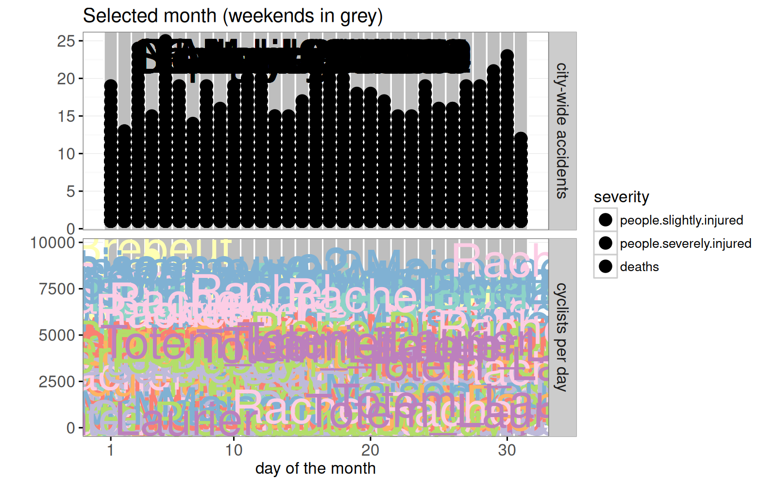
9.4 Chapter summary and exercises
Exercises:
- Change location to a multiple selection variable.
- Add a plot for the map to the data viz.
- On the map, draw a circle for each location, with size that changes based on the
countof the accidents in the currently selectedmonth. - On the
MonthSummaryplot, add a background rectangle that can be used to select themonth. - Remove the
MonthSummaryplot and add a similar visualization as a third panel in theMonthFacetplot.
Next, Chapter 10 explains how to visualize the K-Nearest-Neighbors machine learning model.