# Newton's root-finding method
```{r setup, echo=FALSE}
knitr::opts_chunk$set(fig.path="Ch15-figures/")
```
Roots of a function `f(x)` are values `x` such that `f(x)=0`. Some
functions `f` have an explicit expression for their roots. For
example:
* the linear function `f(x)=b*x+c=0` has a single root `x=-c/b`, if b
is not zero.
* the quadratic function `f(x)=a*x^2+b*x+c=0` has two roots
`x=(-b±sqrt(b^2-4*a*c))/(2*a)`, if the discriminant is positive
`b^2-4*a*c>0`.
* the sin function `f(x)=sin(a*x)=0` has an infinite number of roots:
`pi*z/a` for all integers `z`.
However, there are some functions which have no explicit expression
for their roots. For example, the roots of the Poisson loss
`f(x)=a*x+b*log(x)+c` have no explicit expression in terms of common
mathematical functions. (actually it has a solution in terms of the
[Lambert W function](https://www.wolframalpha.com/input/?i=a*x+%2Bb*log%28x%29%2B+c%3D0)
but that function is not commonly available) This goal of this chapter
is to create an interactive data visualization that explains
[Newton's method](https://en.wikipedia.org/wiki/Newton%27s_method) for
finding the roots of such functions.
Chapter outline:
* We begin by implementing the Newton method for the Poisson loss, to
find the root which is larger than the minimum. We create several
static and one interactive data visualization.
* We then suggest an exercise for finding the root which is smaller
than the minimum.
## Larger root in mean space {#larger-root}
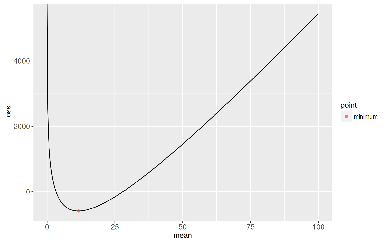
We begin by defining coefficients of a Poisson Loss function with two
roots.
```{r}
Linear <- 95
Log <- -1097
Constant <- 1000
loss.fun <- function(Mean){
  Linear*Mean + Log*log(Mean) + Constant
}
(mean.at.optimum <- -Log/Linear)
(loss.at.optimum <- loss.fun(mean.at.optimum))
library(data.table)
loss.dt <- data.table(mean=seq(0, 100, l=400))
loss.dt[, loss := loss.fun(mean)]
opt.dt <- data.table(
  mean=mean.at.optimum,
  loss=loss.at.optimum,
  point="minimum")
library(animint2)
gg.loss <- ggplot()+
  geom_point(aes(mean, loss, color=point), data=opt.dt)+
  geom_line(aes(mean, loss), data=loss.dt)
print(gg.loss)
```
Our goal is to find the two roots of this function. Newton's root finding
method starts from an arbitrary candidate root, and then repeatedly
uses linear approximations to find more accurate candidate roots. To
compute the linear approximation, we need the derivative:
```{r}
loss.deriv <- function(Mean){
  Linear + Log/Mean
}
```
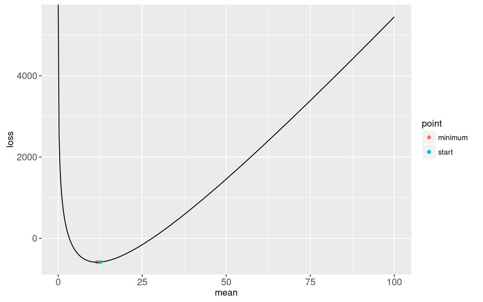
We begin the root finding at a point larger than the
minimum,
```{r}
possible.root <- mean.at.optimum+1
gg.loss+
  geom_point(aes(
    mean, loss, color=point),
    data=data.table(
      point="start",
      mean=possible.root,
      loss=loss.fun(possible.root)))
```
We then use the following implementation of Newton's method to find a
root,
```{r}
iteration <- 1
solution.list <- list()
thresh.dt <- data.table(thresh=1e-6)
while(thresh.dt$thresh < abs({
  fun.value <- loss.fun(possible.root)
})){
  cat(sprintf("mean=%e loss=%e\n", possible.root, fun.value))
  deriv.value <- loss.deriv(possible.root)
  new.root <- possible.root - fun.value/deriv.value
  solution.list[[iteration]] <- data.table(
    iteration, possible.root, fun.value, deriv.value, new.root)
  iteration <- iteration+1
  possible.root <- new.root
}
root.dt <- data.table(point="root", possible.root, fun.value)
gg.loss+
  geom_point(aes(possible.root, fun.value, color=point),
             data=root.dt)
```
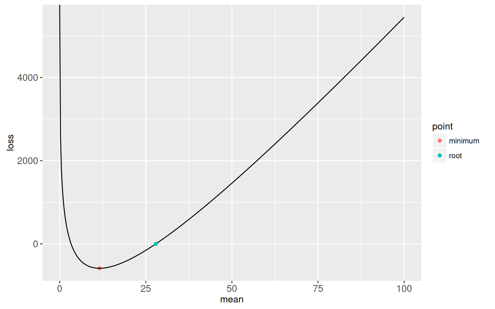
The plot above shows the root that was found. The stopping criterion
was an absolute cost value less than `1e-6` so we know that this
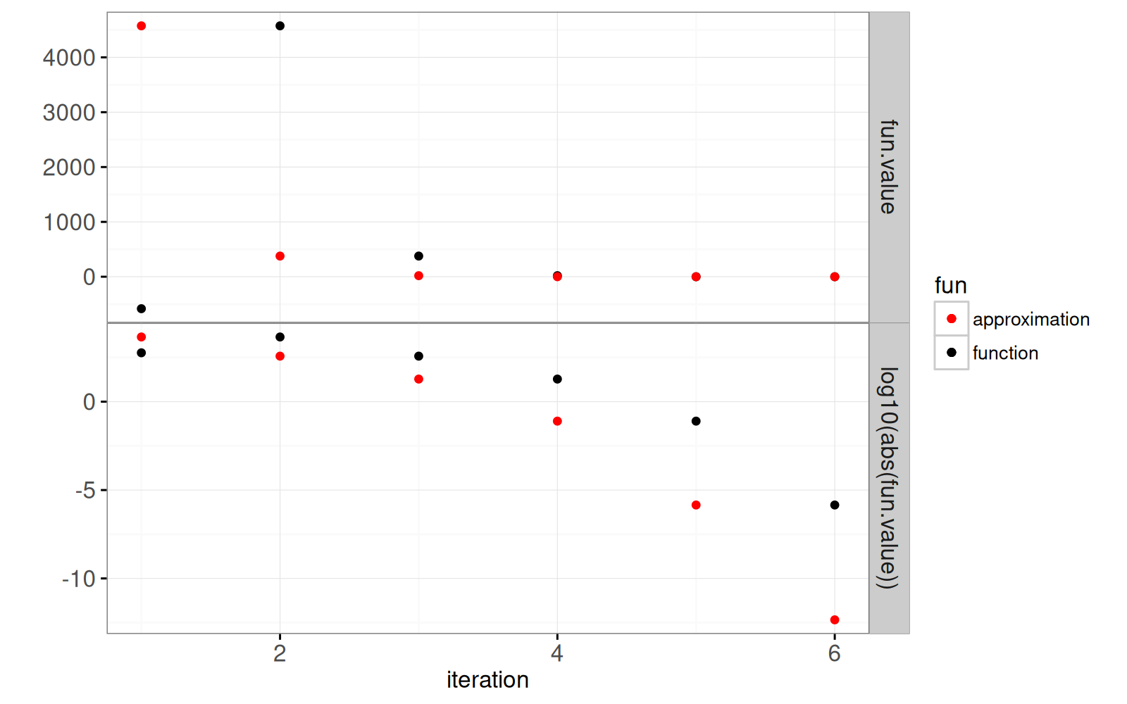
root is at least that accurate. The following plot shows the accuracy
of the root as a function of the number of iterations.
```{r}
solution <- do.call(rbind, solution.list)
solution$new.value <- c(solution$fun.value[-1], fun.value)
gg.it <- ggplot()+
  geom_point(aes(
    iteration, fun.value, color=fun),
    data=data.table(solution, y="fun.value", fun="function"))+
  geom_point(aes(
    iteration, log10(abs(fun.value)), color=fun),
    data=data.table(
      solution, y="log10(abs(fun.value))", fun="function"))+
  scale_color_manual(values=c("function"="black", approximation="red"))+
  geom_point(aes(
    iteration, new.value, color=fun),
    data=data.table(solution, y="fun.value", fun="approximation"))+
  geom_point(aes(
    iteration, log10(abs(new.value)), color=fun),
    data=data.table(
      solution, y="log10(abs(fun.value))", fun="approximation"))+
  theme_bw()+
  theme(panel.margin=grid::unit(0, "lines"))+
  facet_grid(y ~ ., scales="free")+
  ylab("")
print(gg.it)
```
The plot above shows a horizontal line for the stopping criterion
threshold, on the log scale. It is clear that the red dot in the last
iteration is much below that threshold.
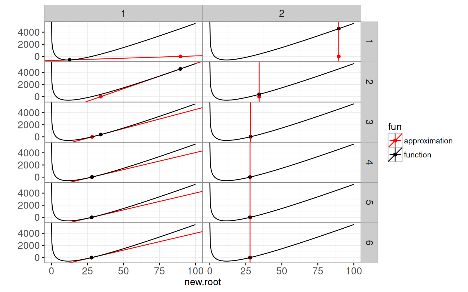
The plot below shows each step of the algorithm. The left panels show
the linear approximation at the candidate root, along with the root of
the linear approximation. The right panels show the root of the linear
approximation, along with the corresponding function value (the new
candidate root).
```{r}
## y - fun.value = deriv.value * (x - possible.root)
## y = deriv.value*x + fun.value-possible.root*deriv.value
ggplot()+
  theme_bw()+
  theme(panel.margin=grid::unit(0, "lines"))+
  facet_grid(iteration ~ step)+
  scale_color_manual(values=c("function"="black", approximation="red"))+
  geom_abline(aes(
    slope=deriv.value, intercept=fun.value-possible.root*deriv.value,
    color=fun),
    data=data.table(solution, fun="approximation", step=1))+
  geom_point(aes(
    new.root, 0, color=fun),
    data=data.table(solution, fun="approximation"))+
  geom_point(aes(
    new.root, new.value, color=fun),
    data=data.table(solution, fun="function", step=2))+
  geom_vline(aes(
    xintercept=new.root, color=fun),
    data=data.table(solution, fun="approximation", step=2))+
  geom_point(aes(
    possible.root, fun.value, color=fun),
    data=data.table(solution, fun="function", step=1))+
  geom_line(aes(
    mean, loss, color=fun),
    data=data.table(loss.dt, fun="function"))+
  ylab("")
```
It is clear that the algorithm quickly converges to the root. The
following is an animated interactive version of the same data viz.
```{r Ch15-viz}
animint(
  time=list(variable="iteration", ms=2000),
  iterations=gg.it+
    theme_animint(width=300, colspan=1)+
    geom_tallrect(aes(
      xmin=iteration-0.5,
      xmax=iteration+0.5),
      clickSelects="iteration",
      alpha=0.5,
      data=solution),
  loss=ggplot()+
    theme_bw()+
    scale_color_manual(values=c(
      "function"="black",
      approximation="red"))+
    geom_abline(aes(
      slope=deriv.value, intercept=fun.value-possible.root*deriv.value,
      color=fun),
      showSelected="iteration",
      data=data.table(solution, fun="approximation"))+
    geom_point(aes(
      new.root, 0, color=fun),
      showSelected="iteration",
      size=4,
      data=data.table(solution, fun="approximation"))+
    geom_point(aes(
      new.root, new.value, color=fun),
      showSelected="iteration",
      data=data.table(solution, fun="function"))+
    geom_vline(aes(
      xintercept=new.root, color=fun),
      showSelected="iteration",
      data=data.table(solution, fun="approximation"))+
    geom_point(aes(
      possible.root, fun.value, color=fun),
      showSelected="iteration",
      data=data.table(solution, fun="function"))+
    geom_line(aes(
      mean, loss, color=fun),
      data=data.table(loss.dt, fun="function"))+
    ylab(""))
```
## Comparison with Lambert W solution {#lambert}
The code below uses the Lambert W function to compute a root, and
compares its solution to the one we computed using Newton's method.
```{r compare-lambert}
inside <- Linear*exp(-Constant/Log)/Log
root.vec <- Log/Linear*c(
  LambertW::W(inside, 0),
  LambertW::W(inside, -1))
loss.fun(c(
  Newton=root.dt$possible.root,
  Lambert=root.vec[2]))
```
For these data, the Lambert W function yields a root which is slightly
more accurate than our implementation of Newton's method.
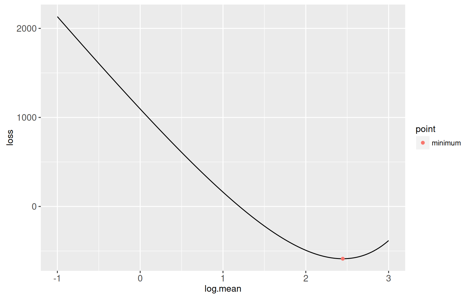
## Root-finding in the log space {#log-space}
The previous section showed an algorithm for finding the root which is
larger than the minimum. In this section we explore an algorithm for
finding the other root (smaller than the minimum). Note that the
Poisson loss is highly non-linear as mean goes to zero, so the linear
approximation in the Newton root finding will not work very
well. Instead, we equivalently perform root finding in the log space:
```{r logloss}
log.loss.fun <- function(log.mean){
  Linear*exp(log.mean) + Log*log.mean + Constant
}
log.loss.dt <- data.table(
  log.mean=seq(-1, 3, l=400)
)[
, loss := log.loss.fun(log.mean)]
ggplot()+
  geom_line(aes(
    log.mean, loss),
    data=log.loss.dt)+
  geom_point(aes(
    log(mean), loss, color=point),
    data=opt.dt)
```
**Exercise:** derive and implement the Newton method for this
function, in order to find the root that is smaller than the
minimum. Create an animint similar to the previous section.
## Chapter summary and exercises {#Ch15-exercises}
In this chapter we explored several visualizations of the Newton
method for finding roots of smooth functions.
Exercises:
* Add a title to each plot.
* Add a size legend to the first plot (black points larger than red), so that we can see when red and black have the same value.
* Add a `geom_hline` to emphasize the loss=0 value in the second plot.
* Add a `geom_hline` to emphasize the stopping threshold in the first
plot.
* Turn off one of the two legends, to save space.
* How to specify smooth transitions between iterations?
* Instead of using iteration as the animation/time variable, create a
new one in order to show two distinct states/steps for each
iteration, i.e. the `step` variable in the facetted plot above.
* What happens to the rate of convergence when you try to find the
larger root in the log space, or the smaller root in the original
space? Theoretically it should not converge as fast, since the
functions are more nonlinear for those roots. Make a data
visualization that allows you to select the starting value, and
shows how many iterations it takes to converge to within the
threshold.
* Create another plot that allows you to select the threshold. Plot
the number of iterations as a function of threshold.
* Derive the loss function for
[Binomial regression](https://en.wikipedia.org/wiki/Binomial_regression),
and visualize the corresponding Newton root finding method.
* Refactor `gg.it` code to use only one `geom_point`, instead of the four geoms in the current code. Hint: use `rbind()` to create a single table with all of the data.
Next, [Chapter 16](../Ch16/Ch16-change-point.html) explains how to visualize
change-point detection models.